How to Estimate Carbon Fiber Production Line Cost?
Estimating Carbon fiber production line cost requires more than adding equipment prices. A reliable estimate connects production capacity, material specifications, automation levels, factory conditions, and long-term operating needs. A small pilot line may require different machinery than a continuous industrial line producing aerospace-grade tow. The difference can reach millions of dollars.
This guide explains the main cost drivers through a practical engineering perspective. It considers precursor preparation, stabilization ovens, carbonization furnaces, surface treatment, sizing, winding, quality control, utilities, installation, and workforce training. Each stage affects the final investment. For example, a furnace rated for higher temperatures may increase purchase costs, energy demand, ventilation requirements, and maintenance expenses.
Details matter.
Supplier quotations should identify output per year, energy consumption, included controls, delivery terms, spare parts, and commissioning support. Factory space also deserves careful attention. A production line may need reinforced flooring, cooling water, exhaust treatment, fire protection, and reliable electrical capacity. These items are often overlooked in early budgets.
Real projects rarely match the first spreadsheet. Exchange-rate changes, construction delays, testing failures, and design modifications can affect the final figure. That uncertainty should be acknowledged, not hidden. A credible estimate normally separates capital expenditure from operating expenditure and includes a reasonable contingency allowance. However, contingency percentages should reflect project maturity and technical risk, rather than guesswork.
By comparing supplier data, consulting experienced engineers, and checking performance references, investors can build a more defensible budget. The following sections examine Carbon fiber production line cost step by step, helping readers distinguish essential investment from avoidable expense.
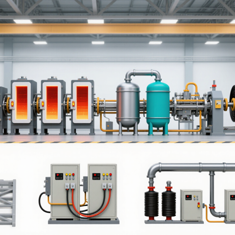
Define Annual Carbon Fiber Capacity: 1,000–5,000 Metric Tons per Year
How to Estimate Carbon Fiber Production Line Cost?
Define Annual Carbon Fiber Capacity: 1,000–5,000 Metric Tons per Year
Annual output is the first cost driver. A 1,000-ton line may use fewer conversion zones and simpler material handling. A 5,000-ton facility needs larger furnaces, parallel processing paths, and stronger utility systems. Capacity is not just a number. It affects building size, energy demand, staffing, maintenance, and storage.
Start with the precursor requirement. Calculate expected fiber yield, production losses, and planned operating hours. A line targeting 1,000 metric tons may need more than 1,300 tons of precursor annually. The exact figure depends on the process route and product grade. Small errors here can distort equipment sizing. They can also weaken the investment estimate.
Break the budget into equipment, installation, utilities, engineering, testing, and commissioning. Include electricity, natural gas, cooling water, ventilation, and waste treatment. These costs can change significantly between regions. I have seen early budgets underestimate furnace installation and electrical infrastructure. That mistake is common. Add a realistic contingency, often 10–20 percent during early planning. Review the model again after pilot trials, because actual yield and line speed may differ from laboratory assumptions. A 5,000-ton target may look efficient on paper, yet idle time can reduce real output sharply. Use both nameplate capacity and expected sellable production when comparing options.
Convert PAN Precursor Demand Using a Typical 40%–50% Carbon Yield
How to Estimate Carbon Fiber Production Line Cost?
PAN precursor demand is a major cost driver in carbon fiber production. A practical estimate starts with carbon yield, usually around 40%–50%. This means 1,000 kilograms of finished carbon fiber may require 2,000–2,500 kilograms of PAN precursor. Use this formula: PAN demand = target carbon fiber output ÷ carbon yield. For example, a line producing 500 tonnes annually needs about 1,000–1,250 tonnes of PAN. The lower yield creates a higher material bill.
Yield is not always measured the same way. Some calculations cover stabilization and carbonization only. Others include trimming, breakage, and off-specification material. This difference can distort a quotation. In practice, I would model three cases: 40%, 45%, and 50% yield. Then compare precursor, electricity, gas, labor, maintenance, and waste costs. A spreadsheet may look precise, but its assumptions may still be weak.
Tips: Ask suppliers how they define yield. Check whether the figure includes startup losses and rejected fiber. Add a realistic operating factor, such as 80%–90% of rated capacity. Early estimates often ignore downtime. That is a mistake. Also test PAN price changes, because a small yield loss can increase annual spending significantly. Keep a separate allowance for utilities and quality control. Forecasts should be practical, not perfect.
How to Estimate Carbon Fiber Production Line Cost? - Convert PAN Precursor Demand Using a Typical 40%–50% Carbon Yield
Planning reference for converting annual carbon fiber output into PAN precursor demand and a preliminary production-line budget.
Target Carbon Fiber Output
(Metric Tons/Year) | Carbon Yield | Required PAN Precursor
(Metric Tons/Year) | Average Carbon Fiber Output
(Metric Tons/Day, 330 Days) | Average PAN Demand
(Metric Tons/Day, 330 Days) | Indicative Installed Line Budget
(USD Million) |
| 500 | 40% | 1,250.0 | 1.52 | 3.79 | 15–30 |
| 500 | 45% | 1,111.1 | 1.52 | 3.37 | 15–30 |
| 500 | 50% | 1,000.0 | 1.52 | 3.03 | 15–30 |
| 1,000 | 40% | 2,500.0 | 3.03 | 7.58 | 25–50 |
| 1,000 | 45% | 2,222.2 | 3.03 | 6.73 | 25–50 |
| 1,000 | 50% | 2,000.0 | 3.03 | 6.06 | 25–50 |
| 3,000 | 40% | 7,500.0 | 9.09 | 22.73 | 65–130 |
| 3,000 | 45% | 6,666.7 | 9.09 | 20.20 | 65–130 |
| 3,000 | 50% | 6,000.0 | 9.09 | 18.18 | 65–130 |
| 5,000 | 40% | 12,500.0 | 15.15 | 37.88 | 100–200 |
| 5,000 | 45% | 11,111.1 | 15.15 | 33.67 | 100–200 |
| 5,000 | 50% | 10,000.0 | 15.15 | 30.30 | 100–200 |
| 10,000 | 40% | 25,000.0 | 30.30 | 75.76 | 180–350 |
| 10,000 | 45% | 22,222.2 | 30.30 | 67.34 | 180–350 |
| 10,000 | 50% | 20,000.0 | 30.30 | 60.61 | 180–350 |
Core calculation: Required PAN precursor = Target carbon fiber output ÷ Carbon yield. For example, producing 1,000 metric tons of carbon fiber requires approximately 2,000–2,500 metric tons of PAN precursor at a 50%–40% yield, respectively.
Typical Cost Allocation for a Greenfield Carbon Fiber Production Line
| Cost Category | Typical Share of Installed Line Budget | Main Cost Drivers |
| PAN precursor preparation and spinning | 20%–30% | Polymer solution preparation, coagulation, washing, drying, and spinning capacity |
| Stabilization ovens | 15%–25% | Oven length, temperature zones, residence time, exhaust treatment, and heat recovery |
| Carbonization furnaces | 25%–40% | Low-temperature and high-temperature furnace capacity, atmosphere control, and energy demand |
| Surface treatment and sizing | 5%–10% | Electrochemical treatment, sizing application, drying, and winding equipment |
| Utilities and environmental systems | 10%–20% | Electricity, cooling water, nitrogen, compressed air, ventilation, and off-gas treatment |
| Installation, commissioning, and quality control | 10%–20% | Mechanical and electrical installation, process control, laboratory equipment, and start-up support |
Estimate Energy OPEX at Approximately 14–20 kWh per Kilogram of Fiber
How to Estimate Carbon Fiber Production Line Cost?
Energy use is a major variable in carbon fiber production line cost. A practical planning range is approximately 14–20 kWh per kilogram of fiber. This estimate includes heating, oxidation, carbonization, surface treatment, and auxiliary systems. It should not be treated as a guaranteed factory result.
For example, a line producing 500 kilograms daily may consume 7,000–10,000 kWh each day. At an electricity price of $0.10 per kWh, daily energy OPEX could reach $700–$1,000. Actual figures depend on furnace insulation, line speed, fiber grade, startup losses, and recovery systems. Small lines often consume more energy per kilogram. That detail is easy to overlook. Production trials are essential before final investment decisions.
Tips: Measure each thermal zone separately. Record power during heating, stable production, shutdown, and material changes. Use at least four weeks of operating data when possible. Include compressed air, cooling water, ventilation, and control equipment in the energy model. A spreadsheet should compare rated power with measured consumption. Rated power alone can mislead. Also, leave room for uncertainty, because early estimates may ignore maintenance downtime, rejected fiber, or seasonal electricity changes.
Model Labor, Maintenance, Yield Losses, and Payback Under Different Scenarios
How to Estimate Carbon Fiber Production Line Cost?
A reliable estimate starts with the production model, not the equipment quotation. Define annual output, tow size, operating days, and planned uptime. Then separate capital cost from operating cost. Include precursor preparation, stabilization, carbonization, surface treatment, sizing, utilities, installation, and commissioning. A line producing 1,000 tonnes annually may require three shifts and several trained operators per shift. Labor costs also include supervision, process engineers, safety staff, training, and absence coverage.
Maintenance is often underestimated. Plan for scheduled inspections, heating elements, rollers, seals, sensors, and control-system support. A practical model may reserve 3–6% of installed equipment value each year, then adjust it using supplier data and local service costs. Yield losses deserve equal attention. During ramp-up, unstable temperatures can create off-specification fiber. A 5% yield loss on expensive precursor material can change the project economics sharply. Real production records are more useful than optimistic quotations.
Build three scenarios: conservative, expected, and improved. Change utilization, labor efficiency, maintenance spending, selling price, and yield in each case. Calculate payback from annual cash flow after energy, labor, maintenance, scrap, and working capital. For example, extending payback from four years to seven years may reveal financing risk. My first spreadsheet ignored cooling-water interruptions; that assumption was wrong. Keep downtime visible. A monthly sensitivity review can show whether output, yield, or energy consumption drives the result. The model should remain editable, because early production rarely follows the cleanest forecast.